Fault diagnosis#
Dataset#
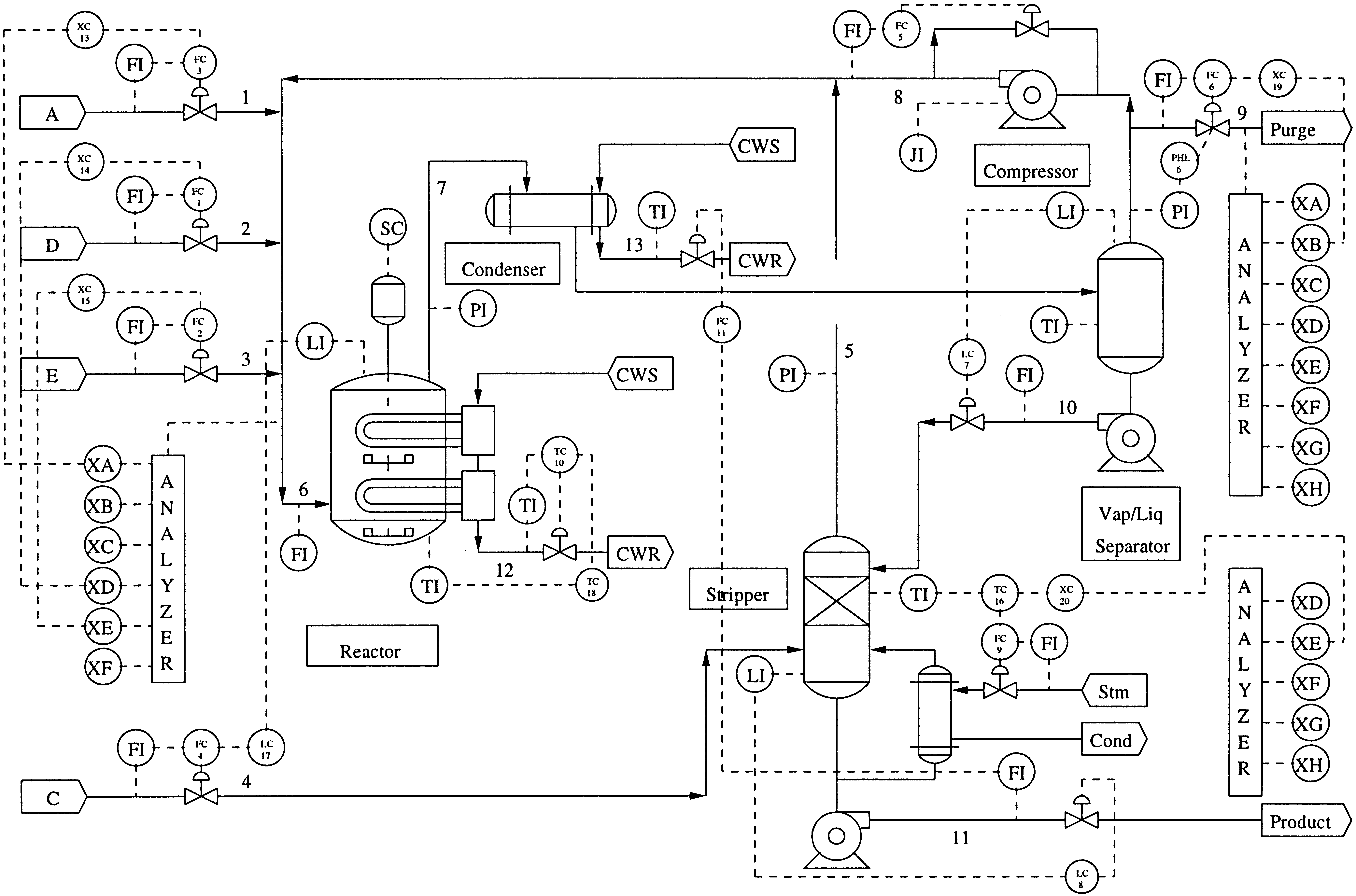
The Tennessee Eastman Process (TEP) [1], created by Eastman Chemical Company, serves as a crucial benchmark in process control and fault detection, mimicking a real chemical plant’s operations and faults (see Figure ref{fig:process_diagram}). The ICE library uses the extended TEP dataset [cite] which consists of 2800 independent simulations of a chemical process. Each run lasts 100 hours, and sensor data is collected at a frequency of 1 time every 3 minutes. Thus, each run consists of 2000 observations. Once started, the process remains in a normal state for 30 hours, after which it goes to a faulty state. The ratio of the training set to the test set is 80/20.
The dataset contains values of 52 chemical process variables: 41 measured variables and 11 manipulated variables. Each moment in time corresponds to a certain state of the chemical process. Faulty conditions are marked with a label corresponding to the fault number from 1 to 28. All other time points are marked with 0.
Task#
In fault diagnosis [2] within the Tennessee Eastman Process (TEP) dataset, the focus is on monitoring a set of process variables to define the operational state of the chemical process and classify them as normal or as one of 28 faults. The data is a multivariate time series consisting of observations \(X_1, X_2 ... X_n\), where \(X_t \in \mathbb{R^d}\) contains the signal values at time point \(t\). Targets are the sequence \(y_1, y_2 ... y_n\), where \(y_t \in \{0,1\}^m\) determines the type of fault at time point \(t\). Then for a sliding window of width \(k\) the function \(f: \mathbb{R}^{d \times k} \rightarrow [0,1]^m\) must be founded, and
where \(l\) is a loss function. The function \(f\) can be approximated using machine learning methods.
Metrics#
In fault diagnosis, several metrics are commonly used to evaluate the performance of models. These metrics help in understanding how well the model is classifying fault types (true positives) and avoiding false alarms (false positives). The choice of metrics often depends on the specific requirements of the task, such as the importance of correct diagnosis versus the cost of false alarms. Common metrics include:
Accuracy measures the overall correctness of the model, calculated as the number of correct predictions divided by the total number of cases.
Correct Diagnosis Rate (CDR) is the number of correctly predicted faulty conditions devided by the number of detected faulty conditions.
Recall (True Positive Rate, TPR) measures the proportion of actual positives (anomalies) correctly identified as such (true positives). It is particularly important in scenarios where missing an anomaly can have serious consequences.
False Positive Rate (FPR) measures the proportion of negative instances that are incorrectly classified as positive (anomalies). A lower FPR is desirable as it indicates fewer false alarms.
References#
The reference results of state-of-the-art papers for the original [1] dataset are presented in Table 1.
Fault |
PCA[3] |
DBN-SVDD[4] |
UN-DBN[5] |
GAN[6] |
MSDAE-TP[6] |
GRU[7] |
|---|---|---|---|---|---|---|
1 |
-/0.98 |
0.02/0.99 |
0.01/0.99 |
0.00/0.99 |
0.01/0.99 |
0.00/1.00 |
2 |
-/0.002 |
0.01/0.07 |
0.02/0.11 |
0.1/0.1 |
0.00/0.22 |
0.00/1.00 |
3 |
-/0.54 |
0.01/0.99 |
0.01/1.00 |
0.06/0.56 |
0.01/1.00 |
0.00/1.00 |
4 |
-/0.22 |
0.01/1.00 |
0.01/1.00 |
0.06/0.32 |
0.01/1.00 |
0.00/1.00 |
5 |
-/0.99 |
0.03/1.00 |
0.01/1.00 |
0.00/1.00 |
0.00/1.00 |
0.00/1.00 |
6 |
-/1.00 |
0.03/1.00 |
0.03/1.00 |
0.00/1.00 |
0.00/1.00 |
0.00/1.00 |
7 |
-/0.96 |
0.02/0.98 |
0.02/0.98 |
0.00/0.98 |
0.02/0.99 |
0.00/1.00 |
8 |
-/0.001 |
0.01/0.01 |
0.01/0.02 |
0.2/0.08 |
0.03/0.04 |
0.00/1.00 |
9 |
-/0.33 |
0.03/0.74 |
0.02/0.82 |
0.00/0.51 |
0.02/0.95 |
0.00/1.00 |
10 |
-/0.2 |
0.01/0.75 |
0.00/0.91 |
0.06/0.58 |
0.03/0.97 |
0.00/1.00 |
11 |
-/0.97 |
0.01/0.99 |
0.01/1.00 |
0.13/0.99 |
0.02/1.00 |
0.00/0.99 |
12 |
-/0.94 |
0.03/0.95 |
0.01/0.95 |
0.02/0.95 |
0.02/0.97 |
0.00/0.99 |
13 |
-/1.00 |
0.02/1.00 |
0.01/1.00 |
0.02/1.00 |
0.01/1.00 |
0.00/1.00 |
14 |
-/0.001 |
0.02/0.14 |
0.02/0.13 |
0.03/0.13 |
0.01/0.39 |
0.00/0.94 |
15 |
-/0.15 |
0.01/0.56 |
0.02/0.64 |
0.2/0.34 |
01/0.92 |
0.00/1.00 |
16 |
-/0.74 |
0.01/0.96 |
0.02/0.98 |
0.02/0.91 |
0.02/0.98 |
0.00/1.00 |
17 |
-/0.88 |
0.03/0.90 |
0.01/0.89 |
0.02/0.90 |
0.01/0.94 |
0.00/1.00 |
18 |
-/0.14 |
0.02/0.59 |
0.03/0.98 |
0.01/0.12 |
0.02/1.00 |
0.00/1.00 |
19 |
-/0.31 |
0.01/0.82 |
0.02/0.87 |
0.00/0.58 |
0.01/0.92 |
0.00/1.00 |
20 |
-/0.26 |
0.02/0.52 |
0.03/0.50 |
0.06/0.5 |
0.02/0.60 |
-/- |
[1] Reinartz, Christopher, Murat Kulahci, and Ole Ravn. “An extended Tennessee Eastman simulation dataset for fault-detection and decision support systems.” Computers & Chemical Engineering 149 (2021): 107281
[2] Abid, Anam, Muhammad Tahir Khan, and Javaid Iqbal. “A review on fault detection and diagnosis techniques: basics and beyond.” Artificial Intelligence Review 54 (2021): 3639-3664.
[3] Yan, Shifu, and Xuefeng Yan. “Design teacher and supervised dual stacked auto-encoders for quality-relevant fault detection in industrial process.” Applied Soft Computing 81 (2019): 105526.
[4] Yu, Jianbo, and Xuefeng Yan. “Layer-by-layer enhancement strategy of favorable features of the deep belief network for industrial process monitoring.” Industrial & Engineering Chemistry Research 57.45 (2018): 15479-15490.
[5] Yu, Jianbo, and Xuefeng Yan. “Whole process monitoring based on unstable neuron output information in hidden layers of deep belief network.” IEEE transactions on cybernetics 50.9 (2019): 3998-4007.
[6] Yu, Jianbo, and Xuefeng Yan. “Multiscale intelligent fault detection system based on agglomerative hierarchical clustering using stacked denoising autoencoder with temporal information.” Applied Soft Computing 95 (2020): 106525.
[7] Lomov, Ildar, et al. “Fault detection in Tennessee Eastman process with temporal deep learning models.” Journal of Industrial Information Integration 23 (2021): 100216.